Project GitHub repository: iiishop/CASA0025_Project
Project Summary
Our project enables a wide range of users to analyse the walkability of London’s streets and explore specific routes. Rather than imposing a single definition, the application allows users to apply their own walkability criteria.
To support this, we break walkability down into a set of pre-computed parameters for each street segment. Users can then assign their own weights to these parameters based on what matters most to them. These user-defined weights are incorporated into a modified cost function within Dijkstra’s algorithm, enabling the system to compute the most suitable route according to each individual’s preferences.
Problem Statement
There are a number of parameters influencing walking comfort; these are widely discussed in literature (Labdaoui et al., 2021; Bartzokas-Tsiompras, Bakogiannis and Nikitas, 2023; Stutz et al., 2025), and some were integrated into the pedestrian routing applications. For example, ShadeRoute, Heal, and Green Paths, integrate % shade, weather, greenness, air quality and noise data indicators into the route-finding cost function.
The products on the market rarely reflect the multifaceted nature of walkability as a concept, focussing on a few selected indicators. Comprehensive tools like Healthy Streets Index rely on fixed indicator weights and lack interactivity, which limits their ability to reflect individual preferences and definitions of walkability; our application addresses the issues above through a fully interactive London-based route-building prototype.
End User
We identified two main end user groups:
Policy makers and built environment professionals require not only robust, evidence-based data to inform policies and interventions, but also the ability to adjust how walkability is defined, e.g. in response to outputs from community engagement. They also need to observe broader patterns, so street scores are displayed as an interactive overlay that updates as users toggle parameters.
The wider public benefits from tools that help identify optimal walking routes. By toggling parameters, users can tailor the route to their immediate needs. The application’s origin-destination module serves as a proof-of-concept, demonstrating how walkability criteria can be integrated into everyday route-planning tools.
Data
We organised the data by walkability criteria that were used in calculations.
Safety from traffic represented with counts of pedestrian collisions occurred 2023-26 (all injury levels). Several years ensure sufficient density of points. © TfL Source
Richness of historic environment represented with listed buildings as points. © Crown Copyright 2026. Contains Ordnance Survey data © Crown copyright and database right 2026. Released under OGL. Source
Availability of shade, represented by mean % of street covered by shade calculated from England 1m Composite DSM. Environment Agency copyright and/or database right 2022. All rights reserved. Source.
Protection from wind, represented by a combination of mean wind speed (m/s) at 10m and presence of barriers. Global Wind Atlas 3.0, a free, web-based application developed, owned and operated by the Technical University of Denmark (DTU). The Global Wind Atlas 3.0 is released in partnership with the World Bank Group, utilizing data provided by Vortex, using funding provided by the Energy Sector Management Assistance Program (ESMAP). For additional information: https://globalwindatlas.info. Source. Environment Agency copyright and/or database right 2022. All rights reserved. Source
Boundaries of London from London Datastore. © Copyright 2026
Methodology
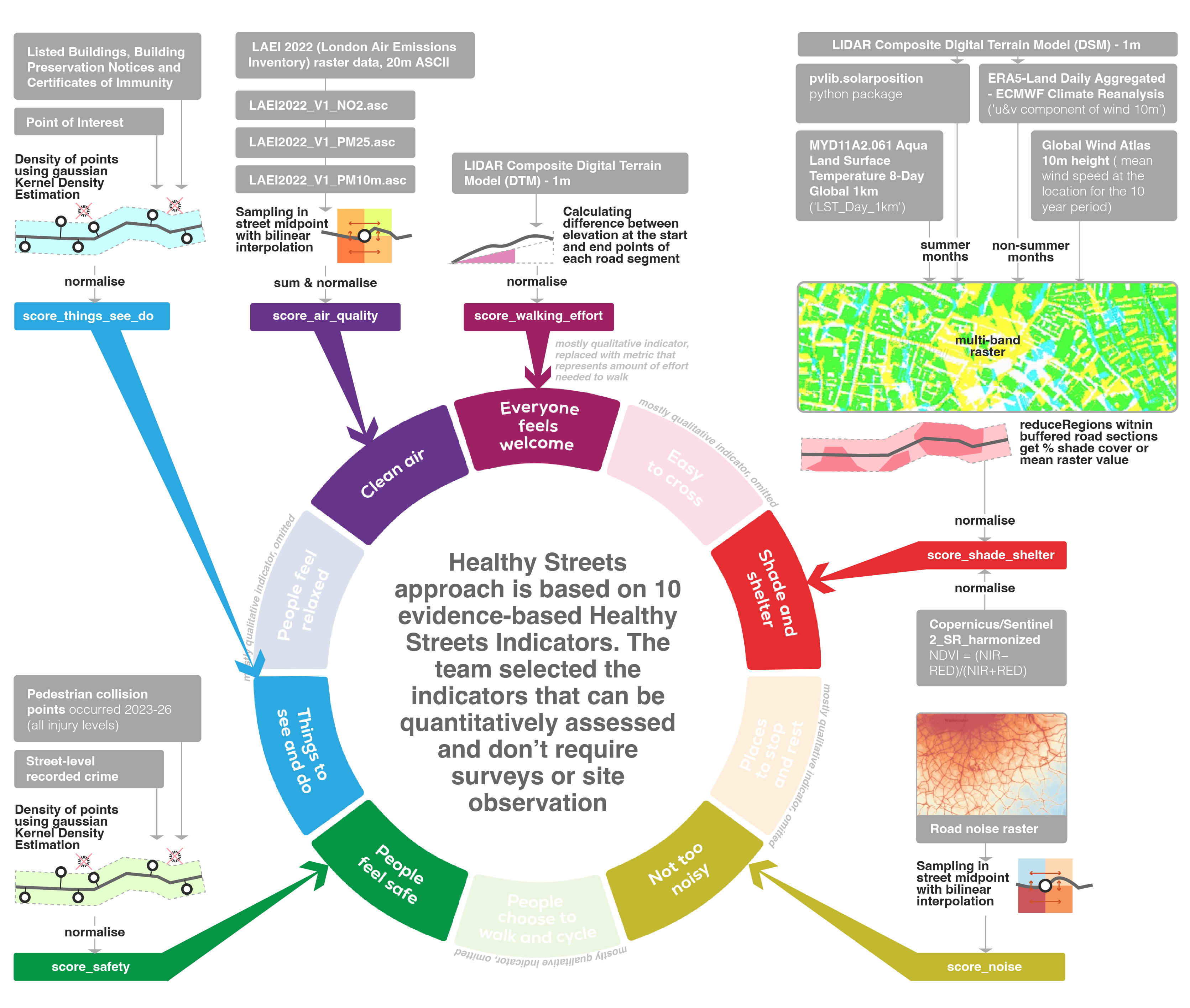
To structure our analysis for London, we adopted the Healthy Streets’ framework, as it is endorsed by the Mayor of London and TfL. We picked quantifiable indicators (as opposed to survey and observation-based), and represented them with composite scores built with raster and point datasets.
We transformed the scores into penalties, and applied them on a graph of walkable networks, which allowed continuous path search across the study area. Using these pre-calculated route-based penalties, the personalised routing cost is defined as a weighted, normalised, and additive cost function:
\[ \Large \begin{aligned} \text{edge\_cost} =\;& w_{\text{length}} \cdot \text{length}_{\text{norm}} \\ &+ w_{\text{safety}} \cdot \text{unsafety}_{\text{penalty}} \\ &+ w_{\text{activity}} \cdot \text{inactivity}_{\text{penalty}} \\ &+ w_{\text{walk}} \cdot \text{walking\_effort}_{\text{penalty}} \\ &+ w_{\text{shade}} \cdot \text{lack\_shade\_shelter}_{\text{penalty}} \\ &+ w_{\text{air}} \cdot \text{polluted\_air}_{\text{penalty}} \\ &+ w_{\text{noise}} \cdot \text{road\_noise}_{\text{penalty}} \end{aligned} \]
Interface
On load the map is showing the default walkability scores plotted. The panel on the left features sliders that allow the user to select their individual preferences; origin-destination block is below. After the preferences and the locations are set, the application is showing two routes: shortest and preferred. As the preferences change, the routes and the general walkability map are changed interactively. For most layers, green indicates more comfortable streets and red indicates less comfortable streets. Street Activity is treated as a hotspot layer, where red highlights more things to see and do.
The Application
The interactive prototype allows users to compare the shortest route with a personalised route, adjust walking-comfort preferences, and explore the network-wide walkability overlay.
Full application (Hugging Face Space): https://ysrei240-comfort-path-final.hf.space
How it Works
Indicator Precomputations
Shade and shelter
This indicator measures whether a street offers shelter from sun in summer and wind during the rest of the year. Script is available here.
Shade cover was modelled using ee.Terrain.hillShadow() with England 1m DSM, which captures buildings, vegetation, and other shadow-casting features. Average summer solar azimuth and zenith were calculated separately using the pvlib package. Mean surface temperature on the hottest day was used to complement the shade metric.
var shadowMap = ee.Terrain.hillShadow({
  image: londonDsmMerc,
  azimuth: 180.02504604372402,
  zenith: 62.63912040279354,
  neighborhoodSize: 100,
  hysteresis: false
});
// Generate the shadow map
var londonShadow = shadowMap.eq(0).rename('shadow')// 1 = shadow, 0 = not shadow
  .toFloat()
  .setDefaultProjection(targetProj);
Wind calculation was simplified by modelling “wind shadow” from prevailing winds using the same approach. Wind direction was derived from ERA5-Land Daily Aggregated horizontal wind vectors for non-summer months. A fixed “zenith” value was used to limit wind-shadow extent, as vertical wind angle could not be robustly estimated. Mean wind speed was used to complement the wind cover metric.
// WIND DIRECTION
var wind = windSource
  .filterBounds(london)
  .filterDate('2025-10-19', '2026-03-19')
  .select(['u_component_of_wind_10m', 'v_component_of_wind_10m'])
  .mean()
  .clipToCollection(london);

// direction wind blows TO
var windTo = wind.expression(
  '(atan2(u, v) * 180 / pi + 360) % 360', {
    u: wind.select('u_component_of_wind_10m'),
    v: wind.select('v_component_of_wind_10m'),
    pi: Math.PI
}).rename('wind_to');

// convert to direction wind comes FROM
var windFrom = windTo.add(180).mod(360).rename('wind_from');

var meanWindFrom = ee.Number(
  windFrom.reduceRegion({
    reducer: ee.Reducer.mean(),
    geometry: london,
    scale: 1000,
    bestEffort: true,
    maxPixels: 1e8
  }).get('wind_from')
);

// 0 = sheltered, 1 = exposed
var windShelterRaw = ee.Terrain.hillShadow({
  image: londonDsmMerc,
  azimuth: meanWindFrom,
  zenith: 39,
  neighborhoodSize: 9,
  hysteresis: false
});

// 1 = wind protected, 0 = not protected
var windProtected = windShelterRaw.eq(0)
  .rename('wind_protected')
  .toFloat()
  .setDefaultProjection(targetProj);
All scores were precomputed in Google Earth Engine by applying ee.Reducer.mean() to the multi-band raster over buffered street segments.
var stacked = londonShadow
  .addBands(surfaceTemp)
  .addBands(windSpeed)
  .addBands(windProtected)
  .clipToCollection(london);


// BATCH PROCESSING BY our_uid
var uidField = 'our_uid';
var batchSize = 80000;
var bufferDistance = 10;   // meters
var exportFolder = 'GEE_Road_Batches';
var exportPrefix = 'roads_stats';

// Check UID range
var minUid = ee.Number(roads.aggregate_min(uidField));
var maxUid = ee.Number(roads.aggregate_max(uidField));

// Number of batches based on UID range
var nBatches = maxUid.subtract(minUid).divide(batchSize).ceil();
print('Number of batches', nBatches);

// Get one batch by UID range: [start, end)
function getBatchByUid(fc, start, end) {
  return fc.filter(ee.Filter.and(
    ee.Filter.gte(uidField, start),
    ee.Filter.lt(uidField, end)
  ));
}

// Buffer roads only for raster extraction; keep original properties
function bufferRoads(fc) {
  return fc.map(function(f) {
    return ee.Feature(f.buffer(bufferDistance)).copyProperties(f);
  });
}

// Run zonal stats for one batch
function computeBatchStats(roadsBatch) {
  var bufferedBatch = bufferRoads(roadsBatch);

  return stacked.reduceRegions({
    collection: bufferedBatch,
    reducer: ee.Reducer.mean(),
    scale: 1,
    crs: 'EPSG:3857',
    tileScale: 8
  });
}
// EXPORT ALL BATCHES
nBatches.evaluate(function(n) {
  minUid.evaluate(function(minVal) {

    for (var i = 0; i < n; i++) {
      var start = minVal + i * batchSize;
      var end = start + batchSize;

      var roadsBatch = getBatchByUid(roads, start, end);
      var statsBatch = computeBatchStats(roadsBatch);

      Export.table.toDrive({
        collection: statsBatch,
        description: exportPrefix + '_' + start + '_' + (end - 1),
        folder: exportFolder,
        fileNamePrefix: exportPrefix + '_' + start + '_' + (end - 1),
        fileFormat: 'CSV',
        selectors: [
          uidField,
          'shadow',
          'surface_temp',
          'wind_speed',
          'wind_protected'
        ]
      });
    }
  });
});
The application below illustrates the 2 core layers generated for “shade and shelter” indicator.
The NDVI was computed with Sentinel2 using the classic approach, and then aggregated into the combined score.
Things to see and do & feeling safe
The point-based scores are constructed using the “hot routes” approach; it was originally developed for crime analysis (Tompson, Partridge and Shepherd, 2009) to better represent route-based concentrations. The script projects points onto street segments, then calculates the density of points based on the gaussian kernel with distance decay, and finally normalises the segment point density by its length. The transformations can be described by the following formula:
\[ \Large \text{KDE}_{\text{segment}} = \frac{ \sum_{i=1}^{n} e^{-0.5 \times \left(d_i / b\right)^2} }{ \text{L} } \]
Where:
\[ \begin{aligned} d_i &= \text{distance from point } i \text{ to street segment (meters)} \\ b &= \text{bandwith, equals 100 meters in the code example} \\ n &= \text{number of points within 100 m} \\ L &= \text{street segment length (meters)} \end{aligned} \]
# Compute KDE score for a road segment from nearby points
for _, point_row in candidates.iterrows():

    dist = geom.distance(point_row.geometry)
    if dist > bandwidth: # Ignore points outside bandwidth radius
        continue
    kernel_weight = _kde_weight(dist, bandwidth, kernel) # Kernel decay
    kde_sum += kernel_weight # Accumulate contribution for segment

kde_segment = kde_sum / segment_length # Normalize by segment length
Each indicator (activity and safety) is aggregated through an unweighted l inear combination of two metrics, aggregated score is rescaled using min–max normalization so that values fall within the predefined range [0,1].
Clean air & noise
The indicators were normalised and treated for missing and extreme values. The normalized indicators were then integrated via a weighted linear combination to derive a composite index for each road segment. Script here.
Walking effort
Slope was derived from a DEM by sampling the start and end points of each road segment and calculating the elevation difference relative to the segment length. This allowed each segment to be described not only by distance but also by the physical effort required to walk along it. The script for this part can be found here.
Network graph and routing
We converted the indicator-enriched network into a graph structure, where each road segment is represented as an edge and intersections as nodes. This allows continuous path search and provides the structural basis for both shortest-path and personalised routing. Instead of rebuilding the graph every time a route is requested, the project uses a cached version (main_graph.pkl), making the system responsive for user interaction.
A limitation of the current framework is that the quality of the personalised route depends heavily on the quality of the segment-level scores produced during preprocessing. Some variables may show highly uneven distributions across the network, which can affect both the visual interpretation of the overlay and the sensitivity of route choice. Additionally, the behavioural realism of pedestrian decision-making is still simplified to a weighted additive structure to keep the model transparent and computationally efficient.
The scripts for this part are stored here.
References
Bartzokas-Tsiompras, A., Bakogiannis, E. and Nikitas, A. (2023) ‘Global microscale walkability ratings and rankings: A novel composite indicator for 59 European city centres’, Journal of Transport Geography, 111, p. 103645. Available at: https://doi.org/10.1016/j.jtrangeo.2023.103645.
Jensen, A., Anderson, K., Holmgren, W., Mikofski, M., Hansen, C., Boeman, L., Loonen, R. “pvlib iotools — Open-source Python functions for seamless access to solar irradiance data.” Solar Energy, 266, 112092, (2023). DOI: 10.1016/j.solener.2023.112092.
How Weighted Overlay works (no date) ArcGIS Pro. ArcGIS Pro. Available at: https://pro.arcgis.com/en/pro-app/latest/tool-reference/spatial-analyst/how-weighted-overlay-works.htm (Accessed: 26 April 2026).
Labdaoui, K. et al. (2021) ‘The Street Walkability and Thermal Comfort Index (SWTCI): A new assessment tool combining street design measurements and thermal comfort’, Science of The Total Environment, 795, p. 148663. Available at: https://doi.org/10.1016/j.scitotenv.2021.148663.
Socharoentum, M. and Karimi, H.A. (2016) ‘Multi-modal transportation with multi-criteria walking (MMT-MCW): Personalized route recommender’, Computers, Environment and Urban Systems, 55, pp. 44–54. Available at: https://doi.org/10.1016/j.compenvurbsys.2015.10.005.
Sprent, R.F. et al. (2024) ‘Multi-Criteria Framework for Routing on Access Land: A Case Study on Dartmoor National Park’, ISPRS International Journal of Geo-Information, 13(4), p. 130. Available at: https://doi.org/10.3390/ijgi13040130.
Stutz, P. et al. (2025) ‘Walkability at Street Level: An Indicator-Based Assessment Model’, Sustainability, 17(8), p. 3634. Available at: https://doi.org/10.3390/su17083634.
Tompson, L., Partridge, H. and Shepherd, N. (2009) ‘Hot Routes: Developing a New Technique for the Spatial Analysis of Crime’, 1(1), pp. 77–96.
Zaragosa, J.J.M. (2025) ‘Using Google Earth Engine to Find Barrier Against Wind Terrain using Wind Direction and Elevation’, Medium, 24 March. Available at: https://medium.com/@junjunzaragosa2309/using-google-earth-engine-to-find-barrier-against-wind-terrain-using-wind-direction-and-elevation-3c5b9fb45ad2 (Accessed: 26 April 2026).